S3.5 Modeling of Laser Machining Process (2)
Models with analytical solutions
Analytical solutions can be got only for simple conditions. We have learned that laser machining process involves many physical processes, such as melting, vaporization, radiation and convection heat transfer. In order to get analytical solutions, usually only pure conduction is considered. In this section, we will go through some of the models with analytical solutions.
The basic 3D PDE for heat conduction in a stationary medium is:
![]()
T is temperature, t is time, ![]() is
the thermal diffusivity. In above equation, we assumed no heat generation and
constant thermal properties, phase changes, convection and radiation are neglected.
We will discuss how to get analytical solutions for different boundary conditions.
is
the thermal diffusivity. In above equation, we assumed no heat generation and
constant thermal properties, phase changes, convection and radiation are neglected.
We will discuss how to get analytical solutions for different boundary conditions.
Heat conduction of an instantaneous point source
In the case of an instantaneous point source, the energy is ![]() and
is applied at t=0 and at the point (x0, y0, z0) of the sample. The BCs are
that at infinity of x, y, z, heat fluxes are zero. The initial condition is
the above mentioned instantaneous point heat source.
and
is applied at t=0 and at the point (x0, y0, z0) of the sample. The BCs are
that at infinity of x, y, z, heat fluxes are zero. The initial condition is
the above mentioned instantaneous point heat source.
This delta function form energy input at the origin of the sample will cause a temperature distribution. It is:
![]()
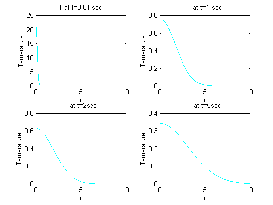
Figure 3.20 The distribution of temperature field at different times (t=0.01, 1, 2 and 5 sec), r is the distance from the center point (x0, y0, z0).
From figure 3.20, you can see the trends of temperature evolution and the temperature distribution in r direction. When t approaches zero, T at r=0 is infinity, as t increases, T decays. The center part has higher temperature than external part.
The time dependent point source
When we assume a time dependent point source, we can still find an analytical solution. In fact, since heat is not a vector quantity, the effects of heat input at different times can be added directly. So for a time dependent heat source, the temperature distribution at any time is the integration of previous temperatures.
The time dependent point source is ![]() ,
which is the energy deposited per unit time at the point (x0, y0, z0). The
BCs are that at infinity of x, y, z, heat fluxes are zero. The initial condition
is the above mentioned point heat source at t=0.
,
which is the energy deposited per unit time at the point (x0, y0, z0). The
BCs are that at infinity of x, y, z, heat fluxes are zero. The initial condition
is the above mentioned point heat source at t=0.
Thus we have the temperature at time t:
![]()
If Q(t) is constant, we have:

Other source shapes
By integrating the point source solution over different areas, the temperature distribution for line sources, Gaussian sources and any other shapes of sources can be found. Also the temporal effect can be considered by the techniques we just used.
For a constant Gaussian beam, P(r,t)=P0 exp[-(r-r0)^2/D^2], where r0 is the center of laser beam, D is the beam diameter.
The solution for the whole area is very complex. The temperature at the center r=r0=0 is:
![]() ,
,
where Rf is the surface reflection for the laser energy.
It is interesting to find an equilibrium temperature at the center when tà inf.
This temperature is:
![]()
This equation provides a rule of thumb for the maximum temperature achievable for a given laser power P0.
 Example:
For AISI 1010 carbon steels, Rf=0.5, D=0.008m, k=63.9W/m.K, compute
the maximum possible temperature for constant laser input at P=10W, 100W and
1000W.
Solution: Using above equation, we found, at P=10W, Tmax=19.56 degree+T0, at P=100W, Tmax=195.6 + T0 degrees, and at P0=1KW, Tmax=1956 degree.
Heat conduction of a moving heat source:
Heat conduction of a moving heat source is of interest because in laser cutting and scribing laser beam is in relative movement to the part. In case of constant scanning velocity, the erosion front and the resulting temperature distribution is constant relative to the coordinate system fixed at the laser beam. In laser drilling however, the laser beam is stationary relative to the part, but the melting front changes with time, so does the temperature field. A steady temperature field simplifies the heat transfer problem. We will discuss this kind of heat conduction in this section.
First we will transfer the time dependence of temperature into spatial dependence using the following quation:
![]()
Where v is the scanning velocity. From this relation, we can rewrite the 3D heat conduction as following:
![]()
In this way we can considered the scanning speed directly in heat conduction analysis.
Assuming a temperature distribution in the following form, the 3D equation can be simplified.
![]()
Where T0 is the initial temperature, f is an unknown function of x,y and z. Take it into the governing equation we have:
![]()
We find that the general heat conduction equation has a simpler form now. For constant scanning velocity, the solution is only spatial dependent.
Next we will study two special conditions.
First, let's consider 1D conduction.
We have:
![]()
The boundary conditions are:
![]() for
for ![]()
We also assume the heat source to be a plane source with a rate of heat q" per unit area:
![]()
Solving the PDE we get:
For x<0,
![]()
For x>0,
![]()
 Example:
For Aluminum, T0=300K, q"=5e7 W/m^2, V=0.01,0.02,0.05 m/s, density=2700
kg/m^3; Cp=903J/kg.K; AA=97.1e-6m^2/s; x=0:1e-4:3e-2;
T=T0+qq*exp(-V*x/AA)/(Cp*density*V1);
The result is as illustrated by figure 3.21. We see for at larger scanning speed, the temperature at the source is lowered.
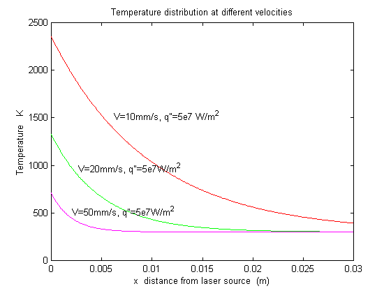
Figure 3.21 Scanning speed and temperature distribution for a 1D moving heat source
For 2D heat conduction problems, we assume that heat flows only in the
x and y-direction, and there is no heat flow in the z direction, so that ![]() ,
the governing equation is:
,
the governing equation is:

In cylindrical coordinates, the governing equation becomes:
![]()
Similarly, the boundary conditions is:
![]() for
for ![]()
![]() for
for ![]()
And we consider a circle area with radius r=(x2+y2)1/2, the heat source take the form:
![]() for
for ![]() ,
here q' is a linear heat source.
,
here q' is a linear heat source.
The cylindrical governing equation with the above boundary equation is known as the modified Bessel function of the second kind and zero order, we denote it as K0(vr/2a ). Then we can express the solution as following:
![]()
 Example:
For Aluminum, T0=300K, q'=1e7 W/m, V=0.01,0.02,0.05 m/s, density=2700 kg/m^3;
Cp=903J/kg.K; AA=97.1e-6m^2/s;
Matlab program for computation:
r=0.01:0.01:0.1; r=r'; theta=0:-pi/50:-pi;
x=r*cos(theta); y=r*sin(theta); R=sqrt(x.^2+y.^2);
K0=besselk(0,V*R/2/AA);
TT=(qq/2/pi/k)*exp(-V*x/2/AA).*K0;
mesh(x,y,TT); title('Temperature distribution with V=0.01m/s, q''=1e7W/m');
xlabel('x (m)'); ylabel('y (m)'); zlabel('Temperature K ');
Some illustrative temperature distributions are shown in figure 3.22 for different scanning speeds, y is the depth in the material, x is the distance from the laser source.
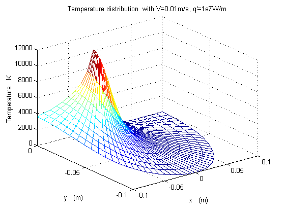
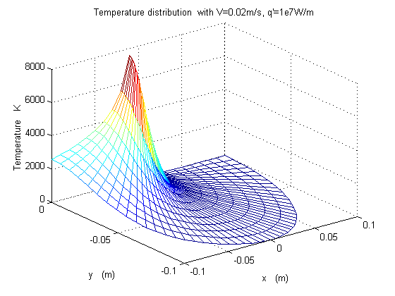
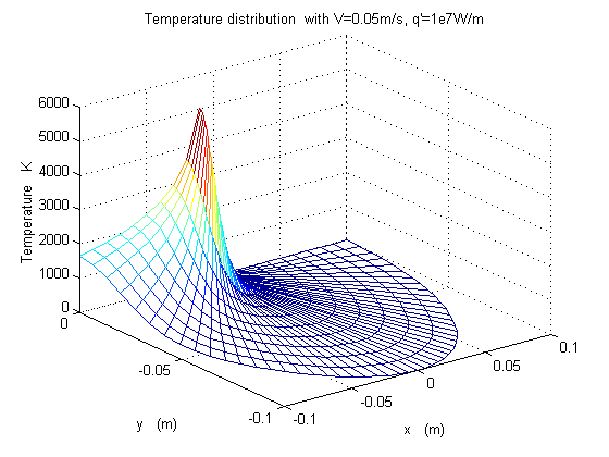
Figure 3.22 temperature distributions are for different scanning speeds, y is the depth in the material
Note: Bessel functions
Bessel functions are solutions to Bessel's differential equation of order NU:
x2 * y'' + x * y' + (x2 - nu2 ) * y = 0
There are several functions available to produce solutions to Bessel's equations in MATLAB. These are:
BESSELJ(NU,Z) Bessel function of the first kind
BESSELY(NU,Z) Bessel function of the second kind
BESSELI(NU,Z) Modified Bessel function of the first kind
BESSELK(NU,Z) Modified Bessel function of the second kind
BESSELH(NU,K,Z) Hankel function
AIRY(K,Z) Airy function
Similarly for the three dimensional case, if we consider a spherical
surface ![]() drawn around the
heat source with radius R=(x2+y2+z2)1/2,
drawn around the
heat source with radius R=(x2+y2+z2)1/2,
Boundary conditions:
![]() for
for ![]()
![]() for
for ![]()
![]() for
for ![]()
And ![]() for
for ![]() ,
here q is a point heat source.
,
here q is a point heat source.
Using spherical coordinate system, the governing equation becomes symmetrical, the solution is only dependent on R:
