S3.6 Modeling of Laser Machining Process (3)

Models with analytical solutions useful for getting some understanding of the physical process involved, but as indicated in last section, analytical solution can only be got for simple conditions. Once complex geometry, boundary conditions, nonlinear phenomena are involved, it will be difficult to get analytical solutions, even if the above mentioned complexity can be described with simple mathematical relations. But the basic laws governing the physical process still apply. In real life, numerical solutions are sought when analytical solutions are not available. Numerical methods are discrete methods, they developed quickly with the development of computer technology. In this section, we introduce you to two kinds of numerical methods, Finite Difference Method and Finite Element Method.

Finite Difference Method

Meshing and Node Index

Unlike analytical solutions, finite difference method computes solutions of the model only at discrete points. Thus one important step in this method is dividing the computation domain into small regions and assigning each region a reference index. Figures 3.23 shows a 2D region, this region is divided into many small meshes. A nodal point is at the center a small region, it has index (m,n), its neighbour points has node index (m,n+1), (m,n-1), (m+1,n), etc. The sum of all these points is known as a nodal network. This step is often called Meshing. The distance between two nodes is called Grid Size. Uniform grid size is used the our figure, but frequently non-uniform grid size are used. Can you speak some reasons for this? In a word, the purpose is to reduce grid number and to increase accuracy. You know the field you computing may change quickly at some parts, while other parts show little changes. So denser grids should be used for the quick change parts, coarser grids are sufficient for slow change areas. Special techniques are used in order to deal with the boundary conditions conveniently. 3D finite difference meshing may also be used, but 2D finite difference meshing is most popular.

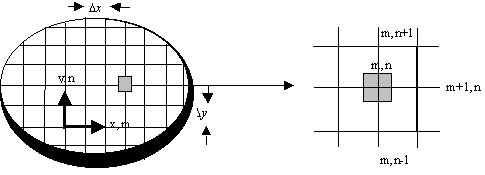
Figure 3.23: Nodal network

Finite Difference Equations:

Accurate numerical determination of the field variable (such as temperature, speed, pressure distributions) requires that the governing equations be written for each nodal point. Taking temperature as example. The resulting equations can then be solved simultaneously for the nodal temperatures. These governing equations are transformed into finite difference form. The key point is how to replace the partial difference with the node values. We denote m-1/2 and m+1/2 as the middle points from node (m,n) along the x-direction. Then the first order partial difference can be expressed using the central difference equation. The temperature gradients in the heat conduction equation can be expressed as follows:

Similarly for the first order partial difference in the y-direction. Then the second order partial difference at node (m,n) to x is :

After substitution, we have:

Using similar logic we can therefore show that:

The change of field variables with time can be transformed by thinking time as the same as a spatial dimension. By convention, we denote time by superscripts such as T⁽ⁿ⁾ as the temperature at time index n.

One guideline for writing the finite difference equations is using the conservation law. If you treat all flux as flowing inward from neighbour points, you can simply write the equation as the sum of inward flux plus the generation of this variable equals zero! We take temperature field for example. This means:

The energy in from neighbour points:

Take these into the energy conservation equation we have:

(4.39)

Following this law, you can easily deal with complex situations.

Let's give you an example.

Example: You are asked to derive the finite difference equation of node (m, n) in figure 3.24. Node (m, n) is on the boundary, there is a heat flux q", there is no heat generation.

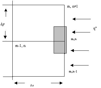
Figure: 3.24 A node with heat flux in on the boundary

Solution:

Using E_in=0 we have

Assume same grid size in x, y direction then we have:

Suppose you have got all the equations for the nodes involved, the next step is choosing suitable method to solve them. There are many methods, such as Matrix Inversion Method which is suitable for small number of equations, Gauss-Seidel Iteration method and the TDMA algorithm. We won't go into detail of these solving techniques. You can refer to books on finite difference computations.

After solving the equations, it is good practice to check whether the numerical solution has been correctly derived. This can be accomplished through substituting the solution into the energy balance equations and check if the balance is satisfied to a high level of precision. If this is not the case then you should check for any possible errors in the formula.

Even if the finite difference equations have been correctly derived and calculated, one should keep in mind that the solution is still an approximation to the real field values. This is due to the finite spacings between nodes and the finite-difference approximations to the governing equations. The level of precision could be increased if the nodal network is refined, ie. being reduced. This would increase the accuracy and the number of nodes in the mean time. Further refinements could result in a situation when the values of no longer matter, thereby making the results grid-independent. These results would provide an accurate and precise solution.

Another method to test the validity of numerical solution is simply to compare numerical solutions with those obtained in an exact solution. This option is rarely exercised primarily because numerical solutions are rarely applied to those problems that possess exact solutions. It is still possible, however, to test one's solution by applying finite-difference procedures to a simpler version of the problem.

Finite Element Methods

When irregular geometry are involved, finite difference method may be inadequate to mesh the computation domain. In this case, Finite Element Methods are often used. In fact, many commercial software use FEM approach because it is more flexible. We can say that Finite Difference Method is point-wise approximations to the governing equations, while Finite Element methods use piecewise or regional approximations.

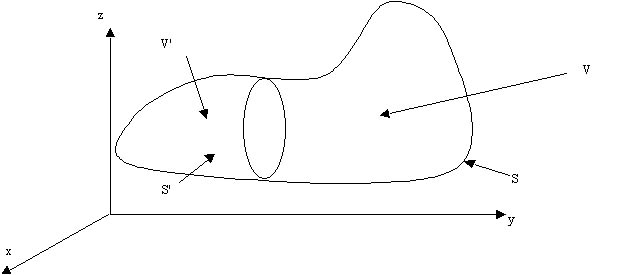
Figure 3.25: Principles of FEM

The finite element method is based on integral minimization. Formulations are based on weighted integrals of a differential equation over a region of space. Consider the domain in figure 3.25, in any part of V the time dependent diffusion equation can be applied. We can integrate this equation over the whole volume v or over any sub-volumes v':

Such volume integrals can be converted into surface integrals, and different profiles can be used to evaluate the surface integral (for example, triangles, squares). The region is first divided in to elements, different elements may contain different number of nodes. The value of the element depends on the selection of the interpolation function. You can think the element value as an weighted average of the element node values. The equations of an element is formulated using the above integral formula. The equations of all the elements are assembled into a larger dimension matrix form. Now choose the field variable f of the element as the weighted average of its nodal points:

Where f _i(t) are quantities defined at the node points, p_i(x) the spatial dependent weight function, N is the number of node of the element. This represents the approximation of the real value. Inserting this approximation into the integral formula, define the residual to be e , we have:

The residual reflects the error between the true value of f and the approximation value of f . If the error is zero, the true solution has been found. This requires that the weighted integral of e to be zero over the entire domain:

i = 1,2,…,N (4-242)

So iterations is carried out, corrections is made to make the error approaches the required value, then the value of f is regarded as converged, the computation moves to next computation cycles.

Figure 3.26 shows a figure from Abaqus FEM stress analysis.

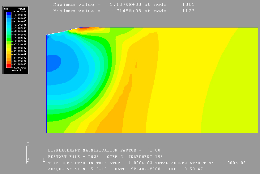
Figure 3.26 Example of FEM

Example: Finite Difference Method Illustration(1D heat transfer)

The fuel element of a reactor is composed of a flat plate (material 1, k1= 100 W/(m C) ) of thickness 60 cms with cladding material (material 2, k2 = 10 W/ (m C) ) of thickness 20 cms bonded to both sides of the plates. Assume the fuel element to have a unit width (1 meter) in the direction normal to the paper. Uniform energy generation of 50,000 Watts per m3 is assumed to take place in material 1 alone. The entire element is immersed in a coolant. The heat transfer coefficient to the coolant is 200 W/(m2 C) with a coolant Tinf of 25 C. We wish to determine the steady-state temperature distributions in the fuel element as well as the cladding. Exploit the symmetry about the centerplane in formulating the problem.

1) Formulate the problem for numerical solution using control volumes. You must decide on where to locate control volume boundaries and where to place the nodes. Use no more than ten nodes in the entire problem.

2) Write a computer program to solve the equations obtained above. This should be a separate subroutine using the TriDiagonal Matrix Algorithm.

3) Validate your program by solving for T(x) for the following test case. Set the cladding conductivity as well as the heat transfer coefficient to be very large values.

You should be able to solve this problem analytically. Compare the numerical results with analytical results for this test case.

4) Solve the actual problem of interest. Plot the temperature distribution in the fuel element. Verify heat conservation for the entire fuel element.

5) Now consider the case of a temperature dependent energy generation term S = 150,000 e-T/400 watts per m3, and T is temperature in degrees C. With all other properties being the same redo the above problem and plot the temperature distribution in the fuel element.

Figure 3.27 1D heat tranfer solutions

Solutions:

See above figure. You can run the following Matlab programs to see the detailed solution. Study this example to get some experience of finite difference method.

Appendix 1:

% heat1d.m

% Steady State Heat Transfer With Heat Generation.

% Wenwu Zhang, 2000.02.14

clear all; format compact;

disp('Part one: Set simulation constant parameters')

K1=100; K2=10;

h1=0; %Convection heat transfer coefficient

h2=200;

Tinf1=25;

Tinf2=25; %temperature in C.

L1=0.3 %L1 is material1 length

L2=0.2 %L2 is material2 length

N1=300

N2=300

N=N1+N2;

disp('Part two: setup geometry related parameters.')

%Use mymesh.m to compute the Xcv positions.

disp('Uneven mesh. Dense near BC.');

[dx1,Xcv1]=mymesh(0.3,N1+1,1,0);

[dx2,Xcv2]=mymesh(0.2,N2,1,0.3);

Xcv=[Xcv1(1:N1),Xcv2];

Xg(1)=Xcv(1);

Xg(2:N)=(Xcv(1:N-1)+Xcv(2:N))/2;

Xg(N+1)=Xcv(N);

Xg;

LXcv(1)=0; LXcv(N+1)=0; LXcv(2:N)=Xcv(2:N)-Xcv(1:N-1);

LXg(1:N)=Xg(2:N+1)-Xg(1:N);

LXgn(1:N)=LXcv(1:N)/2;

LXgp(1:N)=LXcv(2:N+1)/2;

%Set and Compute Kg--K at grid; Kcv--K at cv interface.

Kg(1:N1)=ones(1,N1)*K1; Kg(N1+1:N+1)=ones(size(N1+1:N+1))*K2;

f(1:N)=LXgp(1:N)./LXg(1:N);

Kcv(2:N-1)=1.0 ./( (1-f(2:N-1))./Kg(1:N-2) +f(2:N-1)./Kg(2:N-1) );

Kcv(1)=Kg(1); Kcv(N)=Kg(N+1);

disp('Part Three: Setup Computation Coefficients')

%Moved to loops for future unsteady conditions.

oldTemp=Tinf2*ones(1,N+1); newTemp=oldTemp;

%Source term:

% Since source term is temperature related, it should be renewed inside the iteration.

% Case 1: I1=5e4; afa1=0; I2=0, afa2=0;

I1=5e4; afa1=0; I2=0, afa2=0;

% Case 2: I1=5e4; afa1=0; I2=0, afa2=0;

I1=1.5e5;

afa1=1/400;

I2=0;

afa2=0;

disp('Part 4: Computation iteration')

TempConverge=1e-2;

Terror=1; iterN=1; MaxIteration=100;

while Terror > TempConverge & iterN < MaxIteration

iterN

%Renew nonlinear conefficient S,Sc,Sp, AA.P, b, etc.

%note: if any property vary with time, they can be put into the loop.

AA.E(1:N)=Kcv(1:N)./LXg(1:N);

AA.E(N+1)=0;

AA.W(2:N+1)=Kcv(1:N)./LXg(1:N);

AA.W(1)=0;

Sc(1:N1)=I1*exp(-afa1*oldTemp(1:N1)).*(1+afa1*oldTemp(1:N1));

Sc(N1+1:N+1)=I2*exp(-afa2*oldTemp(N1+1:N+1)).*(1+afa2*oldTemp(N1+1:N+1));

Sp(1:N1)=-afa1*Sc(1:N1)./(1+afa1*oldTemp(1:N1));

Sp(N1+1:N+1)=-afa2*Sc(N1+1:N+1)./(1+afa2*oldTemp(N1+1:N+1));

b(2:N)=Sc(2:N).*LXcv(2:N);

AA.P(2:N)=AA.E(2:N)+AA.W(2:N)-Sp(2:N).*LXcv(2:N);

%Apply left BC:

AA.P(1)=h1+Kcv(1)/LXg(1);

b(1)=h1*Tinf1;

%Apply right BC:

AA.P(N+1)=h2+Kcv(N)/LXg(N);

b(N+1)=h2*Tinf2;

%Call TDMA1D to compute the temperature distribution.

A=AA.P;B=AA.E;C=AA.W;D=b;

newTemp=tdma1d(A,B,C,D);

figure(1); plot(Xg,newTemp,'m');hold on;plot(Xg,newTemp,'g'); plot([Xcv(N1+1),Xcv(N1+1)],[0,400])

title('Temperature distribution in a Two Layer Material');

xlabel('X Location (m)'); ylabel('Temperature (C)'); grid on;

pause(0.5);

Terror=sum(sum(abs(newTemp-oldTemp)))

if Terror <= TempConverge

disp(['Converge at iteration ',num2str(iterN)]);

end

oldTemp=newTemp;

iterN=iterN+1;

end

%Energy Conservation Analysis

Area=1

LeftQin=Kcv(1)*(newTemp(1)-newTemp(2))*Area/LXg(1)

RightQin=Kcv(N)*(newTemp(N+1)-newTemp(N))*Area/LXg(N)

HeatGeneration=sum(I1*exp(-newTemp(1:N1)*afa1).*LXcv(1:N1))*Area+sum(I2*exp(-newTemp(N1+1:N)*afa2).*LXcv(N1+1:N))*Area

EnergyBalance=LeftQin+RightQin+HeatGeneration

hold off;

Appendix 2:

function T=tdma1D(A,B,C,D)

% function T=tdma1d(A,B,C,D)

% TDMA computation for A*T(i)=B*T(i+1)+C*T(i-1)+D

% A,B,C,D are parameters, for 1D, they are (m*1),

% D can be the source part.

% T: T(m,1), is the result, temperature, etc.

% Caution: Make sure B is the coefficients of T(i+1) and C is for T(i-1)!!

% Wenwu Zhang, 2000.02.01, in Columbia University

endI=max(size((A)));

T=zeros(size(A));

startI=1;

P(1)=B(1)/A(1);

Q(1)=D(1)/A(1);

for I=(1+startI):endI

t1=(A(I)-C(I)*P(I-1));

t2=(A(I)-C(I)*P(I-1));

P(I)=B(I)/t1;

Q(I)=(D(I)+C(I)*Q(I-1))/t2;

end

T(endI)=Q(endI);

for I=(endI-1):-1:startI

T(I)=P(I)*T(I+1)+Q(I);

end

Appendix 3:

function [dx,Xcv,Xu,X]=mymesh(length,M,gain,X0)

%function [dx,Xcv,Xu,X]=mymesh(length,M,gain,X0)

%Calculate the mesh position of Control Volum Xcv, velocity Xu and grid points X

% length: the total length will be divided into M points.

% M: total grid points, X0 is the common initial position of Xcv, Xu and X.

% gain: for even distance grid points, gain=1,

% for uneven points: gain>1, from dense to sparse, or gain<1, from sparse to dense

% dx(1+gain+gain^2+gain^3+..+gain^(M-2)=length

% Xcv=Xu, i.e. control volume interface position is the same as the velocity position;

% X(i) the grid position is (Xcv(i)+Xcv(i-1))/2;

% Note: 2*K(i)*K(i-1)/(K(i)+K(i-1)) is harmonic average; Xcv,Xu,X are 1*M vector

% Wenwu Zhang, 1999.10.31, in Columbia University

if nargin==2

gain=1; X0=0;

elseif nargin==3

X0=0;

elseif nargin==4

;

else

error('Input argument number not right!');

end

Xcv(1)=X0;

X(1)=X0;

temp=gain.^(0:M-2);

dx=length/sum(temp);

temp1=dx*cumsum(temp);

Xcv(2:M)=X0+temp1;

Xu=Xcv;

for i=2:M

X(i)=(Xu(i-1)+Xu(i))/2;

end

X(M+1)=length+X0;